
[Updated April 2023: R1.8 of the Cerebras Software Platform now supports image segmentation on 50 megapixel images, up from 25 megapixels in R1.7.]
Convolutional Neural Networks have gained widespread popularity for various Computer Vision tasks in last decade. Accelerating CNNs that work on large images or volumes has been quite a challenging task for computer architects and system designers given the steep compute and memory requirements. At Cerebras, we’re uniquely positioned to accelerate large image CNNs, due to the architectural advantages of wafer-scale integration and our Weight Streaming execution mode. In this blog, we demonstrate our capabilities in this space and elaborate on these advantages.
Introduction
Breakthrough performance achieved with convolutional neural network models (CNNs) for computer vision is what triggered the current “AI summer”. The triggers were larger networks (more layers), new network designs (like ResNet), and fast hardware with which to train these. CNN-based vision models have proved to be useful in autonomous vehicles and robots, agriculture, medicine, and other areas. Most recently, text-based image synthesis – also known as generative AI – based on CNN backbones (Dall-E, Stable Diffusion and Mid-Journey, for example) has been in the spotlight.
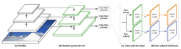
In many CV networks, there is a backbone model that generates feature maps. For example, ResNet serves as the backbone for the RetinaNet [1] object detection network, as shown in Figure 1. Feature maps from the backbone network are then consumed by a subsequent set of layers (task heads) that perform specialized computation. The backbone model, which is often pre-trained on a generic dataset, forms the foundation for the rest of the network. Some common backbones used in CV applications are the ResNet [3] and VGG [4] family of networks.
For image segmentation, the U-Net [2] architecture is often used. The goal of image segmentation is to partition an image into multiple segments or groups of pixels that correspond to different objects or regions. There are different types of segmentation depending on the requirements of the downstream task like semantic segmentation and instance segmentation. A modified form of U-Net is also used in the de-noising step of diffusion models, which are popular for text to image generation (like Stable Diffusion [5] from Stability AI).
Segmentation and classification for large images or volumes stress today’s AI compute systems. They need enough memory to store the weights and activations. For example, the popular 3D U-Net model, when training on 5123 sized volumes requires 64 gigabytes of storage for intermediate activations from the forward pass per image.
To grow memory and compute capacity, implementers have used large clusters of GPUs. But it has proven difficult to split a training job across large clusters and achieve an efficient, stable, successful training run.
The Cerebras Architecture and its advantages
At Cerebras, we believe our platform, the CS-2 system, is built using the only architecture in production that can overcome these challenges:
- The Wafer-Scale Engine (WSE), which powers the CS-2 system, is the world’s largest computer chip. On a single CS-2, we can train a large vision model on large images. This eliminates the need to orchestrate and manage a large GPU cluster. The 40GB of on-chip SRAM and the high-speed, low-latency fabric provide ample memory capacity and performance, and interconnect bandwidth for handling the needs of CNNs. Monolithic training eliminates the problem of sub-linear performance scaling due to inter-chip synchronization, a problem common in large GPU clusters.
- Our Weight Streaming mode of execution stores weights in an external device and streams the weights to the CS-2 on demand. This mode disaggregates compute performance from memory requirements, allowing the compute and the memory components to scale independently to effectively meet an application’s needs. And when one CS-2 is not fast enough or large enough for a challenging use case, we have demonstrated linear performance scaling across multiple CS-2s for data parallel training.
The advantages of the CS-2 present a promising opportunity to accelerate and scale CV models, both model size and image size, with minimal effort. Here are some key advantages for CV models:
- We can fit all the compute and activations required for 2D and 3D segmentation/classification models on a single WSE chip
- The Cerebras Graph Compiler for weight streaming allows scaling from small to large images (2D)/volumes (3D) on the same network architecture, with no extra changes required for work distribution, orchestration, or model code.
- Having all the operator data on a single chip means that bandwidth-bound operations such as normalizers aren’t slowed by having to move activation tensors in and out of the compute hardware from external memory.
We’ll say more about these points later.
How Do CNNs Work?
Before we delve into the details of how we implement CNNs on the Cerebras architecture, it’s worth briefly going over how CNNs work and why they are a good candidate for acceleration.
Convolution operators do most of the work in a CNN. Hence, understanding and optimizing the mapping and performance of a convolution operation is crucial.
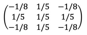
Let’s start by thinking about an image as a 2D array of pixels, where each pixel is a single number. A convolution takes in the image and produces a new image of, usually, the same size. In the output image, the pixel value at a point is a weighted average of the input pixels in a small, normally square neighborhood centered at this same point. The weights used are the same at every point. Thus for example, the output pixel could be the average of the five pixels in the input at the given point and the four neighbors to the north, south, east, and west, minus half the average of the four neighbors in the northwest, northeast, southwest, and southeast directions. This would be a convolution using a 3-by-3 filter with filter coefficients.
You may worry about the output pixels at the edge. What about the neighboring points in the input image that lie outside the image boundary? Some “padding” is used to supply values for these out-of-bounds input pixels; zero-padding is often used, in which these points are ignored.
In real CV applications, an image has another axis, called the feature axis. Each pixel is represented as a vector of values, not a single number. Initially, often it is the 3-vector of red, green, and blue intensities. (At later, downstream layers of a CNN the image dimension, that is the number of pixels on each side, usually shrinks while the feature dimension grows.) A convolution on such an image now computes the feature vector at an output point as a linear function of the neighboring point’s feature vectors. Recall that for any linear function y = f(x) of a vector x, producing a vector y, there is a matrix A such that y = A x, the product of the matrix A and the vector x. If y has dimension m and x has dimension n, then A is an m-by-n matrix; m rows and n columns. Thus, in a 2D convolution with a 3-by-3 filter as above, the filter is defined by nine matrices.
Now imagine that we are working not on a single image but batch of them. As this image batch passes through the network, we apply the convolution operators to them all together, making the feature vectors at a single point into, essentially, and matrix with as many columns as there are images in the batch.
Convolution therefore becomes the following in a 7-dimensional loop nest:
for b in range(batch_size): # SPATIAL
for c in range(input_channels): # SPATIAL
for k in range(num_filters): # TEMPORAL (same as output channels)
for h in range(image_height): # SPATIAL
for w in range(image_width): # SPATIAL
for r in range(R): # TEMPORAL
for s in range(S): # TEMPORAL
output_image[b][h][w][k] += \
input_image[b][h+r][w+s][c] * filter[k][r][s][c]
Figure 3. 7-dimensional loop nest representation of convolution operator.
As you can see, all the loop dimensions are constant. Each output value is a sum of products of input and filter values. The loop ordering is interchangeable. There has been lot of research in industry and academia over the past decade on optimal mapping of the convolution workload to different architectures [6-13].
CNNs on Cerebras
In our weight streaming architecture, convolution has been parallelized by mapping these dimensions either spatially, meaning across different axes of the wafer, or temporally, performing operations one after another rather than in parallel due to the streaming nature of weights. The following diagram (Figure 4) shows the mapping of the spatial dimensions to the two wafer axes. A set of specifications of the different number of PEs across which each of the spatial dimensions are mapped, along with the per PE compute distributions is called a Layout. The Cerebras Graph Compiler takes care of picking the functionally correct and best performing layout choice for all layers in a CNN. The compiler heuristics also take care to make a sensible tradeoff between using the same layouts for each in a set of layers or instead choosing different layouts for consecutive layers, which makes necessary costly activation redistribution between these layers.
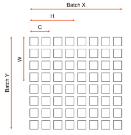
Figure 4. Spatial Data Layout for Multi-Dimensional Convolution tensor on the chip. This is shown for a you example with 8×8 grid of PEs. Actual Cerebras Wafer Scale Chip comprises of 850,000 PEs arranged in a rectangular grid.
Advantages
Large Image Segmentation
The WSE in our CS-2 system has 850,000 processing elements (tiles) in total. We can use all the tiles in the chip to fit one large image. This is much larger than other accelerator architectures out there. This enables our customers to map image classification and segmentation workloads across very large high-resolution images and volumes on to our platform.
With each processing element providing 48 kilobytes for storing pixels, that’s enough to hold a whopping 5 gigapixels (or giga voxels for 3D) on a single chip with each pixel having 3 channels! In theory, this can translate to high resolution 2D images of up to 50,0002 or 3 dimensional volumes of the order of 1,0243.
We have successfully demonstrated mapping and training of segmentation tasks up to 5K2 [now 7k2] resolution on our hardware today. Learn more in this blog post. Stay tuned for updates from us related to further scaling!
Low overhead for traditionally bandwidth bounds operation
Normalization operations like Batch Normalization or Group Normalization are common in CV network architectures, used to solve the problem of covariance shift. Normalization operators are bandwidth bounds operations with very low arithmetic intensity (which is defined as the ratio of compute flops in a workload to the number of bytes of data accessed by it). As a result, these operations can be real utilization killers in GPU based training of CV networks. In the case of data parallel training across GPUs, the problem is exacerbated sometimes due to the need to synchronize between GPUs when performing a batch norm operation (sync batch norm).
In our measurements for training the popular UNET-2D network on a single A100 GPU, the throughput (and utilization) of the training job dropped by up to 50% when Batch Norm or Group Norm was enabled in the workload.
In our WSE-based solution, due to all the availability of activation data for all samples in a batch on chip, a batch norm becomes a low overhead on chip reduction / broadcast operation (Figure 5).
In the upcoming releases we will demonstrate training of CV classification and segmentation networks with Batch or Group Norm layers where the norm overhead is a minimal part of the training workload.
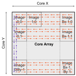
Figure 5. High-level picture of Batch Norm reduction and broadcast on the WSE. Solid lines are reduction paths for mean/variance computation. Dashed lines are broadcast paths. The Reduction phase (solid lines) happens first along the Horizontal direction (orange solid) followed by vertical (purple solid). The Broadcast phase follows, along vertical path (purple dashed) followed by horizontal (orange dashed)
Conclusion
The Cerebras hardware and software platform, which has been designed to meet the growing compute and memory needs of large AI models, can be used to seamlessly accelerate CV models. The potent combination of Wafer-Scale Integration with our Weight Streaming execution mode allows easy scaling to ultra-high resolutions and volumes without any interventions from the user for workload mapping and orchestration.
Manikandan Ananth | February 13, 2023
Try it Today!
Learn More
- More Pixels, More Context, More Insight! – blog about the need for high-resolution computer vision
- UNet Image Segmentation Walkthrough – YouTube tutorial
- UNet Repo – Cerebras Model Zoo
References
- Tsung-Yi Lin, Priya Goyal, Ross Girshick, Kaiming He, Piotr Dollár, “Focal Loss for Dense Object Detection”, arXiv, 2018, https://arxiv.org/abs/1708.02002v2
- Olaf Ronneberger, Philipp Fischer, Thomas Brox, “U-Net: Convolutional Networks for Biomedical Image Segmentation”, arXiv, 2015, https://arxiv.org/abs/1505.04597
- Kaiming He, Xiangyu Zhang, Shaoqing Ren, Jian Sun, “Deep Residual Learning for Image Recognition”, arXiv, 2015 https://arxiv.org/abs/1512.03385
- Karen Simonyan, Andrew Zisserman, “Very Deep Convolutional Networks for Large-Scale Image Recognition”, arXiv, 2015 https://arxiv.org/abs/1409.1556
- Robin Rombach, Andreas Blattmann, Dominik Lorenz, Patrick Esser, Björn Ommer, “High-Resolution Image Synthesis with Latent Diffusion Models”, CVPR 2022, https://arxiv.org/abs/2112.10752 Stable Diffusion
- Vivienne Sze, Yu-Hs in Chen, Tien-Ju Yang, Joel S. Emer, “Efficient Processing of Deep Neural Networks: A Tutorial and Survey”, Proceedings of the IEEE, Vol. 105, No. 12, December 2017, https://www.rle.mit.edu/eems/wp-content/uploads/2017/11/2017_pieee_dnn.pdf
- Hyoukjun Kwon, Ananda Samajdar, Tushar Krishna, “MAERI: Enabling Flexible Dataflow Mapping over DNN Accelerators via Reconfigurable Interconnects”, ASPLOS 2018, https://dl.acm.org/doi/10.1145/3173162.3173176
- Wenyan Lu, Guihai Yan, Jiajun Li, Shijun Gong, Yinhe Han, Xiaowei Li, “FlexFlow: A Flexible Dataflow Accelerator Architecture for Convolutional Neural Networks”, HPCA 2017, https://ieeexplore.ieee.org/document/7920855
- Yu-Hsin Chen, Joel Emer, Vivienne Sze, “Eyeriss: A Spatial Architecture for Energy-Efficient Dataflow for Convolutional Neural Networks”, ISCA 2016, https://ieeexplore.ieee.org/document/7551407
- Mingyu Gao, Xuan Yang, Jing Pu, Mark Horowitz, Christos Kozyrakis, “TANGRAM: Optimized Coarse-Grained Dataflow for Scalable NN Accelerators”, ASPLOS 2019, https://dl.acm.org/doi/10.1145/3297858.3304014
Related Posts
Cerebras Breaks Exascale Record for Molecular Dynamics Simulations
Cerebras has set a new record for molecular dynamics simulation speed that goes…

Supercharge your HPC Research with the Cerebras SDK
Cerebras SDK 1.1.0, our second publicly available release, includes initial…